Picture this: you're in the lab, the spectrophotometer humming, and you need to know how much DNA is in your sample. The Beer‑Lambert law is the shortcut that turns that raw absorbance reading into a real concentration, but the math can feel like a maze.
Does that sound familiar? Maybe you’ve measured a 260 nm absorbance of 0.85 and wondered whether that translates to 50 µg/mL of nucleic acid or something entirely different. That uncertainty is exactly why a solid Beer‑Lambert law example matters.
In our experience at Shop Genomics, we see researchers from university cores to biotech startups constantly juggling sample prep, instrument calibration, and data interpretation. A clear example—plugging the path length, the molar extinction coefficient, and the measured absorbance into the formula—cuts the guesswork and speeds up downstream workflows.
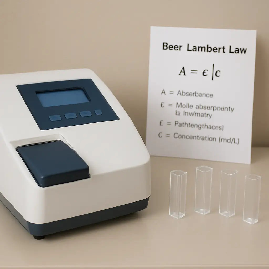
So, how does the calculation actually look? The classic Beer‑Lambert equation, A = ε · c · l, says absorbance (A) equals the molar absorptivity (ε) times concentration (c) times cuvette path length (l). Rearranged, c = A / (ε · l). Simple, right? Yet the choice of ε can be the trickiest part.
Imagine you’re measuring a protein with ε = 33,000 M⁻¹ cm⁻¹ at 280 nm, using a standard 1 cm cuvette, and you record an absorbance of 0.66. Plug those numbers into the rearranged formula and you get c = 0.66 / (33,000 × 1) ≈ 2 × 10⁻⁵ M, which translates to about 1.2 µg/µL. That’s the kind of concrete, repeatable result that lets you move from “maybe” to “definitely” in your experiment design.
What’s the catch? Real samples aren’t always perfectly clear—light scattering, solvent effects, or stray wavelengths can throw off A. That’s why we always recommend a blank measurement with the same buffer and checking the linearity range of your instrument before trusting any single reading.
If you’ve ever felt stuck wondering whether your numbers are off, try running a quick standard curve alongside your unknowns. Plotting absorbance versus known concentrations gives you a visual sanity check and often reveals whether the Beer‑Lambert relationship holds for your specific assay.
TL;DR
In a nutshell, the beer lambert law example shows how plugging your absorbance, path length, and extinction coefficient into A = ε c l lets you instantly convert raw readings into reliable concentrations.
Use a quick standard curve or blank measurement to verify linearity, and you’ll avoid common pitfalls, so your downstream experiments stay on track and reproducible.
Step 1: Understand the Beer‑Lambert Law
Ever stared at an absorbance reading and wondered why it magically turns into a concentration? That's the Beer‑Lambert law doing its quiet work behind the scenes, and getting comfy with it saves you a lot of head‑scratching later.
In plain English, the law says A = ε · c · l. Absorbance (A) is what your spectrophotometer tells you, ε is the molar extinction coefficient (a property of the molecule), c is the concentration you’re after, and l is the path length of the cuvette, usually 1 cm. Rearranged, c = A / (ε · l).
Sounds simple, but the devil’s in the details. If you pick the wrong ε, your calculation is as good as guessing. That’s why we always double‑check the coefficient for the exact buffer conditions and wavelength you’re using.
Here’s a quick mental check: measure a blank with just the buffer, make sure its absorbance is near zero, then record your sample. If the blank reads 0.05, subtract that from your raw A before plugging numbers into the formula. This tiny step prevents systematic over‑estimates.
Let’s walk through a real‑world example that many academic labs face. You’re quantifying a DNA prep at 260 nm, you get an absorbance of 0.85, you’re using a 1 cm cuvette, and the textbook ε for double‑stranded DNA is 50 µg · mL⁻¹ · cm⁻¹. Converting ε to the right units (0.05 mL · µg⁻¹ · cm⁻¹) and applying c = A/(ε · l) gives you about 17 µg/mL. That number tells you whether you need another purification step before downstream PCR.
If you want a step‑by‑step calculator to avoid manual arithmetic, check out our Beer Lambert Law Calculator guide – it walks you through each input and flags values outside the linear range.
But what if your sample isn’t perfectly clear? Light scattering from particulates or pigments can inflate A, making the calculated c too high. A quick way to spot this is to run a dilution series; the absorbance should drop linearly with concentration. If it curves, you’ve got a scattering issue.
Sometimes visualizing the relationship helps. The short video below demonstrates how a standard curve validates the Beer‑Lambert linearity for a protein sample.
Notice how the points line up? That’s the sweet spot where A scales directly with c. When you see deviation, either trim the path length or dilute the sample until you’re back in that linear zone.
A handy tip for CROs and biotech startups is to keep a reference sheet of common ε values right on the bench. That way you can grab the right number without digging through manuals every time.
Looking for a deeper theoretical dive? The team at Ghost Sydney has put together a concise overview of Beer‑Lambert fundamentals that complements the hands‑on tips above.
For a broader perspective on how standardized scales help scientists, see this guide on understanding and using the pencil hardness chart. It’s a neat analogy: just as pencil grades quantify hardness, the Beer‑Lambert law quantifies light absorption.
If you’re curious about how light interacts with other materials, the article on photochromic lenses explains how certain substances change transmission with wavelength – a concept that underpins many absorbance assays.
Bottom line: mastering the Beer‑Lambert law means you’ll trust every absorbance reading, troubleshoot problems before they stall your project, and keep your data reproducible across labs. Next up we’ll show you how to build a reliable standard curve that puts this theory into practice.
Step 2: Set Up the Experiment (Video)
Now that you get why the Beer‑Lambert law matters, it’s time to actually set up a quick experiment you can watch in the video below. The goal? A clean “beer lambert law example” that shows how absorbance changes as you dilute a colored sample.
First, gather your basics: a 1 cm cuvette (plastic or quartz), a pipette, a beaker, and a bright, broadband light source – a simple halogen lamp works fine. If you’re on a tight budget, even a white LED with a diffuser can do the trick.
Step 1 – Choose a relatable sample
We love the tomato‑juice demo because the red pigment (lycopene) gives a vivid color change. It’s cheap, safe, and the absorption peak sits right around 500 nm, perfect for most spectrophotometers. The original study describes the whole workflow in detail, so you can follow that tomato juice experiment if you want extra background.
Step 2 – Prepare a dilution series
Start with pure juice in a small beaker. Then add water to make, for example, 100 %, 50 %, 25 %, 10 %, and 5 % (v/v) solutions. Use a clean pipette for each step and mix well – bubbles ruin the reading.
Tip: label each cuvette with a sticky note so you don’t lose track of which concentration is which.
Step 3 – Blank the spectrophotometer
Fill a cuvette with just the diluent (water or your buffer) and run a blank. The instrument will set that as zero absorbance, removing background light and any cuvette quirks.
Don’t skip this – a missing blank is why many “beer lambert law example” videos look messy.
Step 4 – Record the spectra
Place each cuvette in the light path, one after another, and let the software capture the absorbance at 500 nm (or the nearest wavelength the lamp covers). Most instruments let you save a CSV file with A values – handy for later plotting.
If you see any absorbance above 1.0, dilute that sample further and re‑measure. Staying in the linear range keeps the Beer‑Lambert relationship reliable.
Step 5 – Visual sanity check
Look at the cuvettes side by side. You should see a gradient from deep red (high concentration) to almost clear (low concentration). That visual cue matches the numbers you just recorded.
Now watch the video that walks through each of these steps in real time.
Quick checklist before you wrap up
- All cuvettes are 1 cm path length.
- Blank measurement completed with the same buffer.
- Absorbance values stay between 0.1 and 1.0.
- Data saved in a spreadsheet for plotting A vs. concentration.
- Document any stray bubbles or smudges.
Once you have a tidy data set, plot absorbance on the y‑axis and concentration on the x‑axis. You should see a straight line – that’s your “beer lambert law example” in action. If the line curves at the high end, remember the textbook warning: scattering and inner‑filter effects start to bite.
That’s it! With just a few minutes of prep, you’ve built a reproducible workflow that any lab – from a university teaching bench to a CRO – can adopt. The next step is to use that calibration to convert unknown sample readings into real concentrations, and you’ll be ready for qPCR prep, enzyme kinetics, or any downstream assay.
Step 3: Calculate Concentration from Absorbance
Alright, you’ve got a clean set of absorbance numbers and a straight‑line calibration curve – now it’s time to turn those A values into real concentrations. That moment when the equation finally spits out a number you can actually use is what makes the whole Beer‑Lambert routine worth it.
Plug‑in the numbers
The math is literally one line: c = A / (ε · l). Grab the absorbance (A) you measured for your unknown, pull the molar extinction coefficient (ε) from the datasheet, and confirm the cuvette path length (l), usually 1 cm. Then divide.
Example: your unknown sample reads A = 0.48 at 260 nm. The ε for double‑stranded DNA at that wavelength is 3.0 × 10⁵ L·mol⁻¹·cm⁻¹. Using a 1 cm cuvette, c = 0.48 / (3.0 × 10⁵ × 1) ≈ 1.6 × 10⁻⁶ M. Multiply by the molecular weight of your plasmid (say 2.5 × 10⁶ g mol⁻¹) and you get about 4 µg µL⁻¹. That’s the concrete number you can feed into a downstream qPCR setup.
When the math feels off
Sometimes the result looks too high or low. First, double‑check that you used the correct ε for the exact wavelength. A common slip is borrowing the protein ε = 33,000 M⁻¹ cm⁻¹ for a nucleic‑acid measurement – that will throw the answer off by an order of magnitude.
Second, make sure the absorbance sits in the linear range (0.1–1.0). If A is 1.3, dilute the sample, re‑measure, then back‑calculate by multiplying the concentration you get by the dilution factor.
Quick sanity‑check table
| Step | What to do | Tip |
|---|---|---|
| 1. Record A | Take the absorbance of the unknown at the chosen wavelength. | Use the same cuvette and buffer as the standards. |
| 2. Insert ε & l | Find ε in the reagent’s datasheet; confirm path length. | ε values are wavelength‑specific – don’t guess. |
| 3. Compute c | Apply c = A / (ε · l). | Round to two significant figures for reporting. |
Automation tip for busy labs
If you’re running dozens of samples, most modern spectrophotometers let you export the raw A values as a CSV. Hook that file up to a simple spreadsheet formula (e.g., =A2/($B$1*$C$1) where B1 holds ε and C1 holds l) and let the program fill in concentrations for you. It’s a tiny time‑saver that prevents manual slip‑ups.
For labs that need repeatability across projects, we often suggest saving a “calc sheet” template on your shared drive. Anyone can drop new A values in, hit “Enter”, and instantly see the concentration column update. No one has to re‑type the equation each time.
What to do with the concentration
Now that you have c in moles per liter, convert it to the units your downstream assay expects. Enzyme kinetics might want µM, while a library prep kit might ask for ng µL⁻¹. A quick conversion factor (multiply by molecular weight, then adjust the volume) gets you there.
And don’t forget to log the final number in your lab notebook or electronic LIMS. Include the raw A, ε source, cuvette path, and any dilution factor. That audit trail makes troubleshooting later a breeze.
Wrap‑up checklist
- Absorbance entered correctly?
- ε matches wavelength and sample type?
- Path length confirmed (1 cm or short‑path)?
- Sample within linear range or properly diluted?
- Result recorded with units and calculation notes?
Once you tick all those boxes, you’ve turned a blurry spectrophotometer readout into a reliable concentration – the core of any Beer‑Lambert law example. From there, you can move on to quantifying gene copies, setting up enzyme assays, or any downstream workflow with confidence.
Step 4: Interpret Results and Visualize Data
Now that you’ve got a clean set of absorbance numbers, the next question is – what do they actually mean? Interpreting the raw output is where the Beer Lambert law example turns into a decision‑making tool, not just a number on a screen.
First thing we all do is plot absorbance (A) versus the known concentration of your standards. A straight line tells you the system is behaving linearly – the sweet spot between 0.1 and 1.0 absorbance where most spectrophotometers are most accurate. If the points start to curve, you’re probably hitting scattering or inner‑filter effects, and a dilution is in order.
Step‑by‑step interpretation
1. Export the data. Most modern spectrophotometers let you save a CSV with two columns: concentration and A. Open it in Excel, Google Sheets, or a free Python notebook.
2. Create a scatter plot. Put concentration on the x‑axis, absorbance on the y‑axis. Keep the axes labeled with units (µM or ng/µL) – it saves you a headache later.
3. Fit a linear regression. In Excel, add a trendline and check “Display equation on chart” and “Display R² value.” In Python, numpy.polyfit does the trick in a single line.
4. Evaluate the fit. An R² ≥ 0.99 means your data are solid. Look at the residuals – the differences between observed A and the line. Random scatter around zero is good; a systematic drift hints at a problem with the cuvette or blank.
5. Use the slope to back‑calculate unknowns. The slope (ε · l) is the combined extinction coefficient and path length. Divide any unknown absorbance by this slope to get concentration directly.
6. Add error bars. Propagate the standard deviation of the replicate standards into the y‑error. It gives reviewers confidence that you’ve accounted for variability.
7. Annotate. Write the equation, R², and a note about the blank on the plot. When you share the figure in a lab notebook or a paper, those details prevent endless “what‑did‑you‑use?” questions.
Real‑world example #1 – Academic DNA prep
At a university core, a grad student measured a 260 nm absorbance of 0.78 for a plasmid prep. Their standard curve (0.2, 0.4, 0.6 µg/µL) gave a slope of 3.2 × 10⁻³ µg/µL per absorbance unit and an R² of 0.998. Using the slope, the unknown concentration came out to 0.78 / 3.2 × 10⁻³ ≈ 243 µg/µL. The plotted error bars showed a ±5 % spread, which was acceptable for downstream restriction digests.
Real‑world example #2 – CRO enzyme assay
A contract research lab ran a product assay at 450 nm. Their calibration (0‑50 µM) produced a slope of 0.012 A/µM and an R² of 0.995. An unknown sample gave A = 0.36, so the concentration was 0.36 / 0.012 ≈ 30 µM. Plotting the point on the same graph with a 95 % confidence interval let the client see exactly how the assay performed across the batch.
Pro tip from our team
When you have more than three standards, try a weighted regression – give higher weight to points in the middle of the range where the detector is most linear. It often nudges the slope a few percent, which can be the difference between a successful library prep and a repeat.
Another quick win: color‑code your points by dilution factor. If a 1:10 dilution sits off the line, you instantly know that dilution introduced an error (maybe a bubble or a pipetting slip).
And always keep a copy of the raw CSV alongside the plotted figure. If a reviewer asks for the “original data,” you’ll have it at the click of a button.
So, what should you do next?
Grab your latest CSV, fire up a spreadsheet, and follow the seven steps above. When the plot looks clean and the R² is solid, you’ve turned that “beer lambert law example” into a reliable, visual decision‑tool that anyone in your lab can trust.
Need a visual refresher? Check out this short tutorial that walks through plotting and regression in real time.Beer‑Lambert data interpretation tutorial

Bottom line: interpreting and visualizing your absorbance data isn’t a separate “after‑thought” – it’s the bridge between raw numbers and actionable science. A tidy plot, a clear regression, and a few sanity checks let you move forward with confidence, whether you’re prepping a qPCR library, checking enzyme activity for a biotech client, or teaching undergrads how to trust their spectrophotometer.
Step 5: Common Pitfalls and Tips
We've walked through the math, the blanks, the plots – now it's time to look at the stuff that trips people up. Even a tiny slip can turn a perfect beer lambert law example into a confusing mess.
Pitfall #1: Ignoring the linear range
It sounds simple, but many of us push the spectrophotometer past 1.0 absorbance. When A climbs above that sweet spot, the detector starts to saturate and the relationship between A and concentration bends. The result? Your calculated concentration looks way too low. The fix? Keep every standard and unknown between 0.1 and 1.0, then back‑calculate using the dilution factor.
Pitfall #2: Using the wrong cuvette path length
We all reach for the first cuvette we see, but short‑path cuvettes (0.2 cm, 0.5 cm) need their length entered into the equation. Forgetting to adjust l gives you a concentration that's off by a factor of two or five. A quick visual check – the label on the cuvette or a note in your lab notebook – saves you from that headache.
Pitfall #3: Skipping the blank or using the wrong buffer
Imagine you measured a blank with pure water, but all your samples sit in Tris‑EDTA. The background absorbance from the buffer will be baked into every reading, inflating your A values. Always blank with the exact same solution you use for your standards and unknowns.
Pitfall #4: Overlooking light scattering
Colored or particulate samples scatter light, especially at high concentrations. That extra scatter shows up as an apparently higher absorbance, even if the true chemical absorption is unchanged. Dilute until the solution looks clear, then re‑measure. If you still see a curve on the plot, consider a different wavelength where scattering is lower.
Pitfall #5: Relying on a single ε value
Extinction coefficients can vary with temperature, pH, and even the manufacturer’s lot. Using a generic ε from a paper without confirming it matches your exact conditions can shift your results by 10‑20 %. When possible, run a small standard curve with a known concentration of the same material you’re measuring – that way the slope tells you the effective ε*l for your setup.
Quick tip: Keep a “pitfall log”
Every time you notice something off – a bubble, a stray fingerprint on the cuvette, a sudden jump in R² – jot it down. Over weeks of experiments you’ll see patterns, and future runs will be smoother. A one‑line note in your lab notebook is worth a half‑hour of troubleshooting later.
Tip #1: Double‑check units before you hit calculate
Mixing µg/mL with mg/mL or forgetting to convert nanometers to centimeters is a classic slip. Write the units next to each number on your sheet; the visual cue forces you to pause and verify.
Tip #2: Use a spreadsheet template
Set up columns for raw A, dilution factor, ε, path length, and the formula =A/(ε*L)*Dilution. Once the template is saved, you just copy‑paste new data and let the sheet do the math. No more manual re‑typing errors.
Tip #3: Validate with a second wavelength when possible
If your molecule absorbs at two peaks, run the assay at both wavelengths. The concentrations you calculate should agree within experimental error. If they don’t, you’ve probably hit stray scatter or an incorrect ε.
So, what should you do next? Pull out the CSV you just exported, scan the R² column, and make sure every point sits between 0.1 and 1.0 A. If anything looks fishy, go back, dilute, blank again, and re‑plot. By catching these common pitfalls early, you turn a “beer lambert law example” from a one‑off demo into a reliable workhorse for your lab – whether you’re an academic core facility, a biotech CRO, or a small teaching lab.
Conclusion
We've walked through a full beer lambert law example, from setting up the cuvette to turning raw absorbance into a trustworthy concentration.
Remember the three things that keep your numbers solid: double‑check units, use a fresh blank that matches your buffer, and stay inside the 0.1‑1.0 absorbance window. Those tiny habits stop the common slip‑ups we see in every lab, whether you're a graduate student or a CRO technician.
So, what should you do next? Grab your latest CSV, scan the R² column, and make sure each point sits snugly on a straight line. If something looks off, dilute, re‑measure, and let the math do the heavy lifting.
In our experience at Shop Genomics, having a reliable workflow for the beer lambert law example speeds up downstream steps like qPCR prep or enzyme kinetics. A clean calculation means fewer repeats and more time for the science you love.
Finally, keep a quick checklist on your bench: blank done, path length noted, ε verified, absorbance in range. Tick those boxes and you’ll turn every spectrophotometer reading into a confident data point.
Ready to make your next experiment run smoother? Give the checklist a spin and see how much easier the lab feels.
FAQ
What exactly is a beer lambert law example and why should I care?
In plain terms, a beer lambert law example shows how you turn a raw absorbance number into a real concentration using the equation A = ε · c · l. It matters because every downstream step—qPCR prep, library construction, enzyme assay—relies on knowing how much material you actually have. Skipping this check can mean wasted reagents, failed runs, and extra bench time.
How do I pick the right molar extinction coefficient (ε) for my sample?
The ε value is wavelength‑specific and comes from the supplier’s data sheet or a trusted literature source. Make sure the wavelength you set on the spectrophotometer matches the one listed for ε. If you’re measuring DNA at 260 nm, use the standard 3 × 10⁵ L·mol⁻¹·cm⁻¹; for proteins at 280 nm, grab the value that matches your protein’s tryptophan content.
My absorbance reading is 1.3 AU—should I still use the beer lambert law example?
Ideally keep A between 0.1 and 1.0. Above 1.0 the detector starts to saturate and the relationship bends, giving you a falsely low concentration. Dilute the sample (e.g., 1:10), re‑measure, then multiply the calculated concentration by the dilution factor. That simple step restores linearity and keeps your numbers trustworthy.
Can I use a short‑path cuvette and still apply the same equation?
Absolutely—just plug the actual path length (l) into the formula. A 0.5 cm cuvette will halve the absorbance compared to a 1 cm cuvette, so c = A/(ε · 0.5). Forgetting to adjust l is a common slip that can throw your concentration off by a factor of two or more.
How often should I run a blank, and what should it contain?
Run a blank every time you change buffers, reagents, or cuvette types. The blank should be the exact solvent or buffer you’ll use for your standards and unknowns. This zeroes out background absorbance from salts, plastics, or stray light, preventing systematic over‑estimation of your sample’s A value.
What’s a quick way to check that my beer lambert law example is reliable before moving on?
Create a mini standard curve with at least three known concentrations spanning your expected range. Plot A versus concentration, fit a line, and look for an R² ≥ 0.99. If the points deviate, revisit your ε, path length, or dilution. A clean line tells you the calculation will hold up when you apply it to unknowns.