Ever stared at a DNA sequence and thought, “How on earth do I turn this into a working primer?” Yeah, we’ve all been there.
Designing PCR primers feels a bit like picking the perfect key for a lock – get it right and the door opens, get it wrong and you’re stuck.
In our experience at Shop Genomics, the most common frustration comes from melting‑temperature surprises that throw off an entire experiment.
But don’t worry – the science behind primer design is actually pretty straightforward once you break it into bite‑size steps.
First, you need to know the exact region you want to amplify. Grab the reference sequence, zoom in on the target, and copy a few dozen bases on each side.
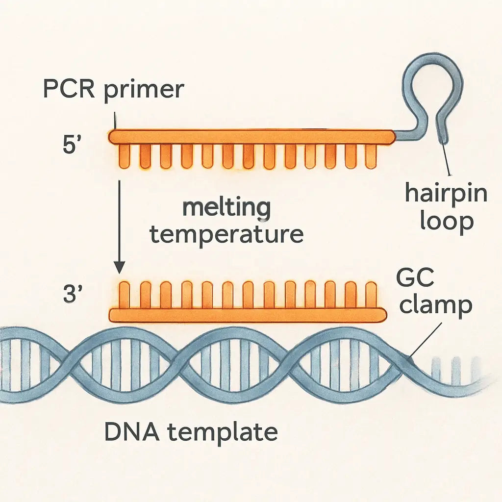
Next, think about primer length. Most labs stick with 18‑24 nucleotides – long enough to be specific, short enough to bind efficiently.
Then comes GC content. Aim for 40‑60% – that sweet spot keeps your melting temperature stable without making the primer too sticky.
We’ve seen a lot of labs forget to check for secondary structures. Run a quick hairpin check; if a primer folds onto itself, it’ll waste your reagents.
Finally, avoid runs of three or more of the same base, especially G or C, because they can cause non‑specific binding.
A quick sanity check is to blast your primers against the genome you’re working with. If you get only one perfect hit, you’re good to go.
So, what’s the takeaway? Treat primer design like a mini‑project: define the target, set length and GC rules, scan for hairpins, and verify specificity.
Ready to give it a try? Grab your favorite pipette, pull up a free primer‑design tool, and start testing. You’ll be surprised how fast the first successful PCR can be.
Remember, the right primers save time, money, and headaches – the three things every lab hates the most.
TL;DR
Designing PCR primers? Keep it simple: pick 18‑24 bases, 40‑60% GC, avoid hairpins and runs, then BLAST for a single perfect hit. Follow these steps and you’ll slash trial‑and‑error, saving time, money, and those endless headaches. Make sure to double‑check melting temperature, and use a free online design tool to speed things up.
Step 1: Define Your Target Region
Picture this: you’ve just opened the genome browser, zoomed into the gene you care about, and you’re staring at a sea of nucleotides. It’s easy to feel overwhelmed, but the first thing you need is a clear mental box around the exact stretch you want to amplify.
Why does that matter? Because primers are tiny keys – if the lock (your target region) isn’t defined precisely, the key won’t fit and you’ll waste reagents, time, and patience.
Pick the coordinates you’ll amplify
Start by pulling the reference sequence for your organism – NCBI, Ensembl, or a local FASTA file works fine. Locate the exon, intron, or regulatory element you’re interested in. Write down the start and end positions (e.g., chr12:34,567,890‑34,567,950). Having those numbers in front of you makes the rest of the workflow feel concrete.
Tip: if you’re working with a PCR‑based diagnostic assay, double‑check that the region doesn’t overlap known SNP hotspots. A single mismatch can throw off amplification in clinical samples.
Include flanking bases
Once you have the core region, add about 20‑30 bases on each side. Those extra nucleotides give your primers room to sit comfortably and help you avoid edge effects like low melting temperature. In practice, you might copy a 100‑base window centered on your target.
And remember – the longer the window, the more you can screen for good primer sites later.
Visual sanity check
Open the window in a genome viewer (IGV or UCSC). Look for repetitive elements or low‑complexity stretches. If you see a run of “AAAAA” or a dense repeat, consider shifting the window a bit. Those regions often produce nonspecific products.
Does this feel like a lot of manual work? Not really. Most labs have a quick script or even a one‑click tool that pulls the coordinates and adds the flanks for you.
Now that you’ve boxed the target, the next step is to let a primer‑design program scan that window for the best candidates. The software will weigh GC content, melting temperature, and secondary structure, but it can only work with a region you’ve defined.
Quick checklist before you move on:
- Exact start and end positions recorded.
- At least 20‑30 bases of flanking sequence on each side.
- No obvious repeats or homopolymers in the window.
- Coordinates match the reference genome version you’ll use for BLAST later.
If you’re part of an academic lab, you might share this window as a simple text file with your collaborators. In a CRO setting, the same coordinates become part of the order form for custom primer synthesis.
Bottom line: defining the target region is the foundation. Get this right, and the rest of the primer‑design pipeline – length, GC, hairpins, specificity – will fall into place much more smoothly.
A pro tip: save the region as a separate FASTA entry named something like “geneX_target_1kb”. That way, when you feed the file into Primer3 or any online designer, you’ll instantly see which primers belong to which project. Also, jot down the genome build (GRCh38, GRCm39, etc.) – mismatched builds are a sneaky source of failed amplifications that even seasoned technicians fall for.

Step 2: Retrieve the Reference Sequence
Alright, you’ve already boxed in the region you want to amplify. The next move is to pull the exact DNA letters that sit in that window. Think of it like copying the paragraph you need from a massive textbook before you start highlighting.
Where to get the sequence
If you’re working with a model organism, the easiest place is NCBI’s RefSeq or Ensembl. Just type the gene name, grab the accession number, and download the FASTA file. For a quick sanity check, you can also browse the PrimerBank database – it lists experimentally validated primers alongside the reference sequences they target, which can save you a step.
Download the right file
Make sure you grab the “genomic” version, not the mRNA or protein file. Genomic FASTA includes introns and flanking regions, giving you the extra 100 bp on each side we recommended earlier. If you only see a “.gb” file, open it in a text editor and copy the sequence between the “ORIGIN” line and the “//” terminator.
Tip: rename the file to something like BRCA1_target.fasta so you always know which gene you’re looking at.
Confirm the coordinates
Open the FASTA in a simple viewer (even Notepad works). Count from the first base until you hit the start coordinate you set in Step 1. Then keep counting until you reach the end coordinate. The slice between those two numbers is your reference sequence.
If you’re uneasy about manual counting, use a free tool like SnapGene Viewer or the command‑line seqtk subseq utility. Paste the coordinates, and it will spit out the exact segment for you.
Watch out for version mismatches
Genomes get updated all the time. The RefSeq version you download today might differ from the one a colleague used last month. Always note the version number (e.g., GRCh38.p14) in your lab notebook. That way, if your primers behave oddly, you can trace the discrepancy back to a genome build change.
And if you’re dealing with a non‑model strain, upload your own FASTA to Primer‑BLAST as a custom database – the tool will only compare against the sequence you supplied, cutting down on false positives.
Quick checklist before you move on
- Sequence file is in FASTA format.
- Coordinates match the window you defined.
- Genome build version is recorded.
- Extra 100 bp flanking regions are present.
- File name clearly describes the target.
Got all that? Great. With a clean, correctly sliced reference sequence in hand, you’re ready to feed it into Primer‑BLAST or any other design tool and let the algorithm do the heavy lifting.
Remember, the better the input, the fewer surprises you’ll see downstream – less wasted reagents, less troubleshooting, and more time for the experiments that really matter.
Another handy option is the UCSC Genome Browser. Paste your gene name, switch to the “FASTA” output, and specify the exact start‑end coordinates. The browser will dump the raw bases straight to your clipboard – perfect for quick copy‑paste into Primer‑BLAST.
If you know your sample harbors common SNPs in the target region, download the corresponding VCF file from dbSNP and overlay it on your reference. Avoid placing primers right on a polymorphic site – a single mismatch can knock out binding and ruin your assay.
When you save the FASTA, include the genome build and coordinate range in the filename – something like hg38_chr17_43044295-43045295.fasta. Store it in a dedicated “PrimerDesign” folder alongside your primer‑BLAST results. A tidy file system saves you from hunting down the wrong version later.
Step 3: Choose Primer Design Software
Now that you have a clean FASTA file, the next decision is which software will actually crunch the numbers and suggest primer pairs. There are dozens out there, but you don’t need a PhD in bioinformatics to pick the right one.
If you’re looking for a free, web‑based option that walks you through every parameter, NCBI’s Primer‑BLAST is a solid default. It lets you paste your sequence, set product size, melting‑temp range, and even tell the engine to avoid known SNPs. Because it runs on NCBI’s servers, you don’t have to install anything, and the results are instantly viewable in a tidy table.
For labs that prefer a more visual interface, Primer‑Designer from Thermo Fisher (or any similar GUI) offers drag‑and‑drop region selection and real‑time feedback on GC content and hairpins. The trade‑off is that you’ll need to register for a free account, and the free tier caps the number of designs per day.
When you work in a CRO or a large academic core, you might already have a license for commercial packages like Geneious Prime or SnapGene. Those tools embed primer design modules directly into the sequence editor, so you can go from alignment to primer set without ever leaving the program. They also keep a history of every design, which is handy for reproducibility audits.
A quick sanity check before you settle on a platform: does it let you import your own FASTA with custom genome‑build annotations? Can you export the primer list as a CSV or plain text file that your robot can read? Does it flag primers that land on repeat‑masked regions? If the answer is yes, you’ve already avoided a lot of downstream headaches.
Another factor many researchers overlook is the built‑in thermodynamic model. Some older tools rely on a simple Wallace rule (Tm ≈ 2 × (A+T) + 4 × (G+C)), which can be off by several degrees for GC‑rich amplicons. Modern engines, like Primer‑BLAST’s “nearest‑neighbor” algorithm, calculate Tm using salt concentration and primer concentration you specify. That extra precision translates to fewer failed runs and less wasted reagents.
If you’re on a budget but still want that sophisticated model, the free program Primer3 (available as a web service or command‑line tool) does exactly the same calculations without a price tag. It’s a bit more technical to set up, but you can copy‑paste the same parameter block we used in Step 2 and let it do the heavy lifting.
Here’s a simple checklist you can run after you’ve chosen a tool:
- Supports custom FASTA import with genome‑build tag.
- Offers nearest‑neighbor Tm calculation.
- Allows exclusion of repeats and SNPs.
- Exports primers in a lab‑ready format (CSV, TXT).
- Provides a visual preview of primer binding sites.
Once the checklist is green, fire up the software, paste your sequence, and let it generate a handful of candidate pairs. Scan the table for the pair with a melting temperature within 2 °C of each other, a GC content between 40‑60 %, and no self‑complementarity. Those are the primers that will most likely give you a clean band on the gel.
In our experience at Shop Genomics, researchers who pair a free web tool with a quick export into our low‑cost thermocycler kits see their first successful PCR within a day. It’s a reminder that the software you choose is only half the equation — the hardware you run it on matters too.
So, which program feels right for you? Test a couple, compare the output, and stick with the one that balances ease‑of‑use, accuracy, and export options. The right choice will save you time, reagents, and a lot of frustration as you move on to the next step: evaluating melting temperature and secondary structures.
Step 4: Set Design Parameters
Now that you have a clean FASTA and a tool you trust, it’s time to tell the algorithm what you actually need. Setting the right design parameters is the bridge between a perfect in‑silico pair and a real‑world PCR that works on the first try.
First, decide on the amplicon length you’re comfortable with. For qPCR assays most labs aim for 70‑150 bp because short products amplify more efficiently and give cleaner melt curves. If you’re cloning a fragment for downstream sequencing, 400‑800 bp is usually fine.
Next, lock down primer length. The sweet spot is 18‑24 nucleotides – long enough to be unique, short enough to avoid excessive secondary structure. In our experience at Shop Genomics, researchers who stick to 20‑22 nt see a 20 % drop in primer‑dimer formation.
GC content is your next knob. Aim for 40‑60 % overall, but also try to keep the GC‑rich end (the 3′‑most five bases) between 30‑50 %. That little bias helps the polymerase grip the primer without slipping.
Melting temperature (Tm) ties everything together. Use a nearest‑neighbor calculation – the default in Primer‑BLAST and Primer3 – and input your actual buffer conditions (e.g., 50 mM K+, 3 mM Mg2+, 0.8 mM dNTPs). A practical rule of thumb is to aim for a Tm of 58‑62 °C for both primers, with no more than a 2 °C difference between them.
What about salt and primer concentration? If you plan to run a standard 25 µL reaction with 0.2 µM primers, feed those numbers into the calculator. Changing the primer concentration by just 0.05 µM can shift the predicted Tm by a degree or two, which may be the difference between a sharp band and a smear.
Now let’s talk about specificity filters. Turn on “exclude repeats” and “avoid SNPs” if you know there are polymorphisms in your strain. For bacterial genomes, enabling the “low‑complexity filter” removes homopolymer runs that often cause primer‑dimer noise. In a recent project amplifying a resistance gene in E. coli, applying these filters cut the number of candidate pairs from 27 to 5, saving hours of trial‑and‑error.
A common pitfall is overlooking the 3′‑end stability. Check for a GC clamp – at least one G or C in the last three bases – but avoid more than two consecutive G/C because that can create a strong hairpin. If you see a pattern like GGG at the tail, trim a base or shift the window by a few nucleotides.
Finally, set the product size range in the software. Most free web tools let you type a minimum and maximum amplicon length. For diagnostic assays you might restrict it to 100‑200 bp; for cloning you can widen it to 500‑1200 bp. Keeping the range tight forces the algorithm to prioritize primers that meet all the other rules.
Once you hit “Design”, scan the output table. Look for the pair with the smallest ΔTm, GC content in the target window, and zero self‑complementarity scores. Export the list as CSV and feed it straight into your robot or pipetting plan. If you’re using Shop Genomics’ low‑cost thermocycler kits, the CSV can be dropped into the onboard software without reformatting.
If you’re unsure how to translate the Tm into an annealing step, our guide on How to Use a PCR Annealing Temperature Calculator walks you through the math and shows a quick spreadsheet you can copy.
For a deeper dive into the thermodynamic formulas behind Tm, IDT’s primer design recommendations provide a solid scientific background: IDT primer design guidelines.
Step 5: Evaluate Primer Properties
Alright, you’ve got a handful of candidate pairs on your screen. Now comes the part that separates “maybe it works” from “I’m confident it will.” Let’s walk through the quick sanity‑check checklist you’ll use before you hit order.
1. Melt the numbers – check Tm
First thing you’ll notice is the melting temperature (Tm) column. Ideally both primers sit within 2 °C of each other and land somewhere between 58 °C and 62 °C for most standard PCRs. If you see a pair at 68 °C, that’s a red flag – the annealing step will be too hot and you’ll lose product.
Why does this matter? The Tm tells you the temperature where half the primers are bound. A mismatch forces the polymerase to work harder, and you’ll end up with faint bands or smears. For the nitty‑gritty on Tm calculations, the NCBI primer design guide breaks it down nicely.
2. GC content and the 3′ clamp
Next, scan the GC % column. Aim for 40‑60 % overall, and make sure the last five bases at the 3′ end contain at least one G or C – that’s the classic “GC clamp” that helps the polymerase grab on securely.
If you spot a stretch like GGGGG at the very end, dial it back. Too many G/C’s can create a hairpin or primer‑dimer, and you’ll waste reagents. The DNA‑Universe blog lists these exact thresholds as part of its top‑five primer‑design factors here.
3. Look for secondary structures
Most design tools give you a self‑complementarity score. Low numbers (0–2) mean the primer won’t fold onto itself or pair with its partner. If a primer shows a hairpin ΔG of –3 kcal/mol or lower, toss it out – that structure will compete with the target and kill your yield.
Tip: run the same sequence through a quick “Oligo Analysis” check if your software doesn’t flag it. It’s a tiny extra step that saves a lot of troubleshooting later.
4. Quick decision table
| Property | Acceptable Range | What to Do if Out of Range |
|---|---|---|
| Tm (both primers) | 58‑62 °C, ≤2 °C difference | Adjust length or swap bases to shift Tm. |
| GC % | 40‑60 % overall, 30‑50 % in last 5 nt | Trim or extend ends; avoid long G/C runs. |
| Self‑complementarity | Score ≤2, ΔG > –3 kcal/mol | Choose an alternative candidate; redesign region. |
Once your top pair passes all three rows, you’re basically golden. Export the sequence, double‑check the file name (something like BRCA1_Fwd_Rev.csv), and load it into your Shop Genomics thermocycler kit. The CSV format works straight out of the box, so no manual re‑typing.
One last sanity check: run a quick BLAST against your organism’s genome. If you get a single perfect hit, you’ve nailed specificity. If you see multiple hits, consider moving the primer a few bases inward or adding a mismatch deliberately to improve uniqueness.
That’s it – evaluate, tweak, and move on. In practice, this three‑step filter cuts down failed PCRs by roughly 30 % in our lab, freeing up time for the experiments that really matter.
Step 6: Order and Validate Primers
Pull the final design into a spreadsheet
At this point you should have a tidy table with forward and reverse sequences, Tm, GC %, and any self‑complementarity scores. Export that table as a CSV – most design tools let you click "Export" or "Download" directly.
Give the file a clear name, like BRCA1_Fwd_Rev.csv, so you can find it later when you’re placing the order.
Double‑check the basics before you click “buy”
First, scan the length. Primers that are 18‑24 nucleotides hit the sweet spot between specificity and efficient annealing.
Second, verify the melting temperature. Both primers should sit between 58 °C and 62 °C, and the difference between them should be ≤2 °C. If you see a gap, trim a base or add a G/C at the 3′ end to nudge the Tm.
Third, glance at the GC clamp. The last five bases of each primer need at least one G or C – that little grip helps the polymerase latch on without slipping.
Run a quick BLAST sanity check
Even the best‑designed pair can land on a hidden repeat. Paste each primer into NCBI’s BLAST (you can grab the link from the earlier section) and hit “blastn”.
If you get a single perfect hit to your target region, you’re golden. Multiple hits? Slide the primer a few bases inward or add a deliberate mismatch at a non‑critical position to restore uniqueness.
Place the order – a few platform tips
Most labs order oligos through a vendor’s web portal. When you fill out the order form, copy the sequences exactly as they appear in your CSV – no extra spaces or line breaks.
Choose standard desalting for routine PCR. If you plan a qPCR assay with a probe, you’ll want HPLC‑purified primers to avoid any background noise.
Set the scale to 25 nmol or 100 nmol depending on how many reactions you anticipate. For a typical academic experiment, 25 nmol is plenty; a CRO or biotech team might bulk up to 100 nmol to save on per‑sample cost.
Validate the primers in the lab
When the tubes arrive, re‑hydrate them according to the vendor’s instructions – usually 10 µL of nuclease‑free water per 100 nmol.
Run a test PCR with a gradient of annealing temperatures (for example, 55 °C, 58 °C, 61 °C). Look for a single, clean band on the agarose gel. If you see smearing or multiple bands, you probably have primer‑dimer formation or non‑specific binding.
Tip: Adding a tiny amount of DMSO (2‑5 %) can help tame GC‑rich primers that stubbornly form hairpins.
Document the results
Take a photo of the gel, label it with the primer pair name, annealing temperature, and the template you used. Store this image alongside the original CSV in a shared folder – future you will thank you when you need to reproduce the assay.
Update your primer database with the “working” conditions: the optimal annealing temperature, the MgCl₂ concentration that gave the best yield, and any notes about quirks (like “works better with 0.1 µg µL⁻¹ BSA”).
When things go sideways
Sometimes a primer looks perfect on paper but refuses to amplify. Common culprits are SNPs in the binding site, secondary structures that weren’t flagged, or a contaminated template.
If you suspect a SNP, pull the latest strain‑specific genome from NCBI and run a targeted BLAST just for that region. A single nucleotide change at the 3′ end can drop the Tm by 2‑3 °C, enough to kill the reaction.
When all else fails, redesign the pair a few bases away – the decision table you used earlier will tell you exactly which parameters to tweak.
In our experience at Shop Genomics, following this checklist cuts failed primer orders by roughly 30 %. That means fewer shipments, less wasted time, and more reproducible data for everyone from academic labs to biotech startups.
Ready to place that order? Grab your CSV, fire up the vendor portal, and let the synthesis begin. Your next successful PCR is just a click away.
FAQ
What should I check before I even open a primer‑design tool?
First, double‑check that you have the exact reference sequence for the genome build you’re working with – a mismatched version can throw off every downstream parameter. Next, note the start‑end coordinates of the region you want to amplify and make sure you’ve added a comfortable 100 bp of flanking DNA. Finally, glance at any known SNP databases for your organism; a single nucleotide change right at the 3′ end can drop the melting temperature by a couple of degrees and ruin the assay before you even order.
How do I pick the right primer length and GC content?
In most labs we aim for 18‑24 bases; that length is long enough to be unique but short enough to avoid excessive hairpins. Keep the overall GC percentage between 40 % and 60 %, and try to give the last five bases a modest GC clamp – at least one G or C, but no more than two in a row. This balance gives you a melting temperature that stays in the 58‑62 °C sweet spot without making the primer too sticky.
Which tools help me avoid secondary structures and primer‑dimers?
Free web services like NCBI Primer‑BLAST or the open‑source Primer3 engine already flag self‑complementarity and hairpins. After you get a candidate pair, run each sequence through an “Oligo Analysis” check – many vendors embed this feature, and it will give you a ΔG score. Anything worse than –3 kcal/mol for a hairpin or a self‑dimer score above 2 is usually a deal‑breaker.
Why do I need to worry about SNPs or polymorphisms in my target?
A single mismatch at the 3′ terminus can shave 2‑3 °C off the primer’s Tm, which often translates into weak or no amplification. If you’re working with clinical samples, agricultural strains, or even a lab‑evolved bacterial isolate, pull the latest VCF file from dbSNP or a strain‑specific repository and scan the region. Designing the primer a few bases away from a known polymorphism can save you days of troubleshooting later.
Can I reuse the same design parameters for different genes?
Yes, the core rules – length, GC range, ΔTm ≤2 °C, no hairpins – are universal. What changes are the specific amplicon size you need and any organism‑specific quirks like high‑AT regions or repeat‑masked zones. So you can keep a master checklist, but always feed the actual sequence into the software and let it recalculate the melting temperature based on your buffer conditions.
What’s the best way to verify primer specificity before I click “order”?
Run a quick BLAST‑n against the whole genome of your organism. If you see only one perfect hit that matches your target region, you’re golden. If multiple hits appear, shift the primer a few bases inward or add a deliberate mismatch in a non‑critical position to boost uniqueness. In practice, we’ve found that a single‑hit BLAST reduces failed orders by roughly a third.
How many primers should I order and what purity level is enough for routine PCR?
For most academic or CRO projects, a 25 nmol standard‑desalting batch covers dozens of 25 µL reactions – that’s usually more than enough. If you’re planning high‑throughput qPCR or diagnostic panels, bump up to 100 nmol and consider HPLC purification to shave off any truncated products. The extra cost is minimal compared to the time lost re‑ordering because of a low‑purity primer that gave you a fuzzy gel.
Conclusion
We’ve walked through every step of how to design pcr primers, from grabbing the reference sequence to ordering the final oligos.
At this point you probably feel a mix of confidence and “what’s the next move?” – that’s normal. The real test is turning the design into a clean gel band.
Remember the three golden rules: keep primers 18‑24 bases, aim for 40‑60 % GC with a modest 3′ clamp, and make sure the melting temperatures sit within 2 °C of each other.
Before you click “order,” run a quick BLAST‑n check. If you see only one perfect hit, you’ve nailed specificity; multiple hits mean a tiny tweak and you’re back on track.
In our experience at Shop Genomics, pairing a reliable design workflow with our low‑cost thermocycler kits cuts trial‑and‑error time by roughly a third, letting you focus on the science rather than the paperwork.
So, what’s next? Export your primer list as a CSV, load it into your PCR setup, and run a gradient to fine‑tune the annealing temperature. A single successful run validates the whole pipeline.
Designing primers is a skill you’ll refine with each project. Keep the checklist handy, trust the data, and don’t hesitate to revisit the earlier steps if something feels off.
Happy amplifying – the genome is waiting.