Ever stared at a tiny glass slide, tried to line up those little squares, and thought, “Is there a faster way?” That moment of frustration is the exact feeling many of us in labs share when we compare a hemocytometer vs automated cell counter.
On hand, the hemocytometer is cheap, reusable, and lets you actually see each cell under the microscope – it feels like you’re doing the counting yourself, which can be reassuring for early‑stage projects or tight budgets. On the other hand, an automated cell counter clicks a button and spits out numbers in seconds, saving you hours when you’re processing dozens of samples a day.
But the choice isn’t just about speed or price. It’s also about accuracy, sample type, and how much hands‑on time you can afford. For example, a researcher juggling tissue culture and flow cytometry might need the consistency of an automated system, while a teaching lab that wants students to learn basic cell biology may prefer the tactile experience of a hemocytometer.
So, what should you ask yourself when you’re stuck between these two options? First, consider the volume of samples you run each week. If you’re counting a handful of plates, the manual method probably won’t slow you down. If you’re handling hundreds of plates in a biotech startup, the automated counter becomes a productivity game‑changer.
Next, think about the cell types you work with. Some automated counters struggle with clumped or fragile cells, whereas a skilled eye on a hemocytometer can still give a reliable estimate. And don’t forget downstream requirements – if your downstream assay demands precise viability percentages, you’ll want the method that gives you the most consistent data.
In the end, the “best” tool is the one that fits your workflow, budget, and scientific goals. Over the next sections we’ll dive into the nitty‑gritty: set‑up tips, error sources, cost breakdowns, and real‑world scenarios from academic labs to large CROs.
Ready to weigh the pros and cons and find the sweet spot for your lab? Let’s explore the details together.
TL;DR
When you weigh hemocytometer vs automated cell counter, think about sample volume, cell type, and how much hands‑on time you can spare in your workflow. If you need speed and reproducibility for high‑throughput projects, an automated counter wins; for low budgets or teaching labs, the hemocytometer stays reliable and cheap.
Understanding Hemocytometers: How They Work
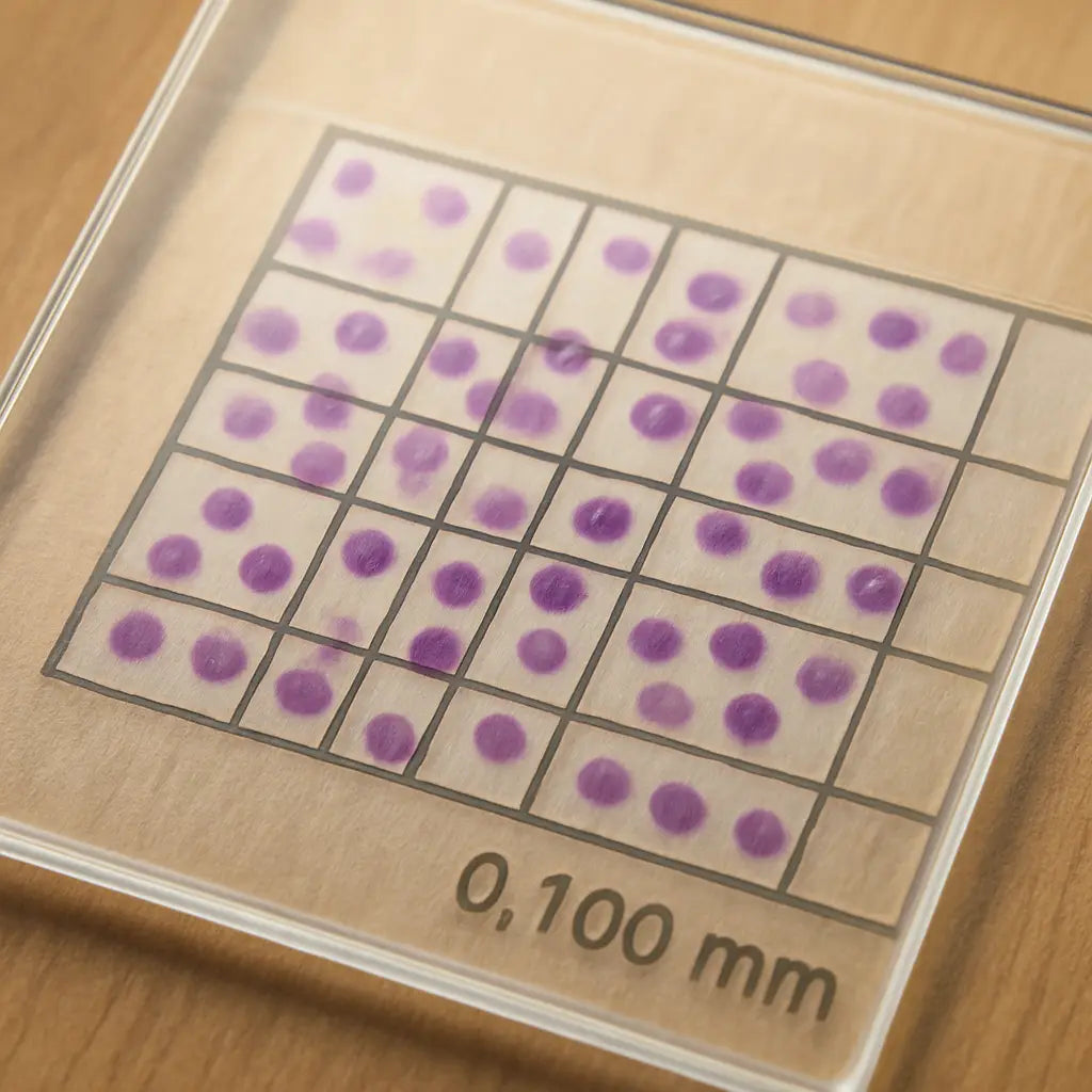
Ever tried to count cells on a tiny glass grid and felt like you were hunting for constellations? That’s exactly what a hemocytometer does – it gives you a defined microscope slide with a series of microscopic squares, each acting as a tiny counting arena. When you load a diluted cell suspension, the cells settle into these wells, and you can literally see and tally them.
So, how does the magic happen? The hemocytometer’s design is based on precise geometry. The most common type, the Neubauer chamber, has a depth of 0.1 mm and a grid of 9 × 9 large squares, each 1 mm². Because the volume over each square is known (0.1 µL), counting the cells in a few squares and multiplying by the appropriate factor gives you cells per milliliter. No software, no calibration curves – just pure optics and a bit of arithmetic.
Key components you’ll meet
First, the cover slip. It’s not just a protective layer; it sets the chamber’s depth. If the slip isn’t perfectly flat, your volume calculations will be off. Next, the grid itself – you’ll notice a central counting area surrounded by larger peripheral squares. The central area is where most labs focus because it balances statistical reliability and speed.
And the microscope? You’ll need at least a 10× objective to resolve individual cells, though many prefer 40× for better discrimination between live and dead cells when you add a stain like trypan blue.
Step‑by‑step workflow
1. Prepare your sample. Dilute the cell suspension to a countable range (usually 10⁴‑10⁶ cells/mL). Too dense, and you’ll waste time chasing overlapping cells; too dilute, and you’ll end up counting empty squares.
2. Mix gently with viability dye. If you’re checking live vs. dead, add trypan blue and let it sit for a minute.
3. Load the chamber. Using a pipette, draw up the diluted sample and gently dispense it into the loading port. Capillary action will draw the fluid across the grid, filling the chamber without bubbles.
4. Let cells settle. Wait about 30 seconds – this lets cells drop to the bottom of the chamber where the grid is etched.
5. Count under the microscope. Count cells in the four corner squares and the central square, applying the standard multiplication factor (usually 10⁴) to get cells per milliliter.
6. Calculate viability. Subtract the blue‑stained dead cells from the total count, then divide by the total to get a percentage.
That’s the core of the manual method. Simple, right? But the devil is in the details – temperature, timing, and even the way you pipette can introduce variance.
For labs that need higher throughput, an automated cell counter handles all those steps with a button press. Still, many academic and teaching labs stick with the hemocytometer because it teaches fundamental concepts and costs just a few dollars.
Here’s a quick visual recap – check out the short video below that walks through loading and counting on a Neubauer chamber.
Notice how the liquid spreads evenly across the grid? That’s the capillary action I mentioned earlier. If you ever see uneven filling, double‑check your pipette tip and make sure the cover slip is clean.
One practical tip we’ve seen work for both research institutes and CROs: use a low‑retention pipette tip when loading the chamber. It minimizes sample loss and ensures the volume you pipette is exactly what ends up in the grid.
If you’re looking for a place to order a reliable hemocytometer, or even a printable version for quick lab backups, JiffyPrintOnline offers custom lab print solutions that can include the grid layout on a polymer sheet. It’s handy for labs that want a disposable option without breaking the bank.
And when you need to validate your counts against a reference standard, the BasinCheck calibration service provides certified reference materials that let you compare manual counts to known concentrations, ensuring your numbers stay trustworthy.
In short, the hemocytometer is a low‑tech, high‑trust tool. Understanding its geometry, mastering the loading technique, and keeping an eye on sources of error will let you extract reliable data – whether you’re a student learning cell biology or a biotech team doing quality control.
Next, we’ll dive into the common sources of error and how to troubleshoot them so your counts stay consistent day after day.
Automated Cell Counters: Technology Overview
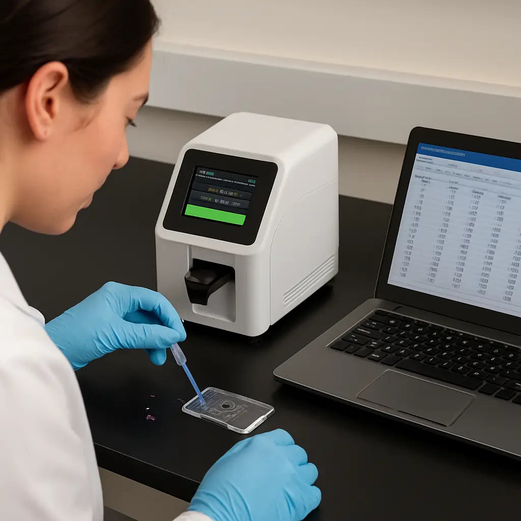
When you first see an automated cell counter on the bench, it can feel like a sci‑fi gadget – a little box with a camera, a light, and a screen that spits out numbers in a flash. The truth is, the technology behind it is a clever mix of optics, fluidics, and software that’s been honed for the exact kind of work labs like yours do every day.
At its core, most modern counters use a bright‑field or fluorescence imaging system. A tiny LED illuminates the sample, and a high‑resolution sensor captures a snapshot of thousands of cells in a single frame. The software then runs algorithms that identify each cell, measure its size, and decide whether it’s alive or dead based on dye exclusion or fluorescence intensity.
How the optics work
Imagine you’re looking at a crowd through a window. If the window is clear and the lighting is even, you can count heads fairly easily. Automated counters replace that window with a calibrated lens and a controlled light source, so every cell is seen under the same conditions. This eliminates the subjective glare or shadows you might get with a microscope.
Some counters, like the Accuris QuadCount™ we stock, offer interchangeable filters. That means you can switch from a simple bright‑field mode for routine viability checks to a fluorescence mode for more specialized assays – for example, detecting GFP‑expressing cells without ever staining them.
Fluidics: moving the sample
The sample handling is just as important as the imaging. Most devices pull a tiny volume (often 10‑20 µL) into a disposable chip or cuvette. The chip has a micro‑channel that spreads the cells into a monolayer, ensuring the camera sees each cell once and only once. This single‑pass design reduces the chance of double‑counting, a common pitfall with manual hemocytometers.
Because the chip is disposable, you don’t have to worry about cleaning or cross‑contamination – a big win for CROs or clinical labs that handle multiple sample types in a day.
Software smarts
After the image is captured, the real magic happens in the software. Machine‑learning models have been trained on millions of cell images, so they can differentiate a live cell from a dead one, spot clumps, and even flag abnormal morphology. The result is a viability percentage, concentration, and often a size distribution all in one click.
One thing we’ve seen work best in biotech startups is to set a “confidence threshold” in the software. If the algorithm isn’t sure about a particular cell, it flags it for manual review. That way you get the speed of automation without sacrificing the trust you’d get from a hemocytometer’s visual confirmation.
So, does the technology really live up to the hype? In practice, labs that switch from manual counting to an automated system often report a 70‑90 % reduction in counting time and a noticeable bump in reproducibility. That’s especially true when you’re processing dozens of plates a day – the time saved adds up fast.
But let’s not forget the nuances. If you’re working with highly clumped stem cells or fragile primary neurons, the counter’s fluidics might shear the cells or miss aggregates. In those cases, a gentle pre‑filter step or a brief vortex can smooth things out before the sample hits the chip.
Another tip: always run a calibration check with a known concentration standard once a week. Most counters have a built‑in routine that compares the measured count to the expected value, and it will alert you if the optics need cleaning or the sensor is drifting.
In short, the technology behind automated cell counters blends precise optics, smart fluidics, and AI‑driven analysis to give you fast, reproducible numbers. Whether you’re an academic lab needing occasional counts or a high‑throughput biotech operation, understanding these components helps you pick the right model and use it to its full potential.
Key Comparison: Accuracy, Speed, and Cost
When you line up a hemocytometer next to an automated cell counter, the first thing you notice is the promise of speed versus the comfort of seeing each cell under the microscope. But does faster always mean better? And how does the price tag really break down when you factor in reagents, maintenance, and labour?
Accuracy: Human Eye vs. Machine Algorithms
Manual counting puts the onus on you to distinguish live cells from debris, red blood cells, or clumps. Even experienced researchers can disagree – a study cited by DeNovix found up to a 90 % reduction in user‑to‑user variability when switching to an image‑based counter.
Automated counters use bright‑field or fluorescence imaging and run the same algorithm on every sample. That means the same cell will be classified the same way every run, as long as the calibration is sound. For labs that work with stem‑cell aggregates or heavily pigmented samples, adding a fluorescent viability stain (AO/PI) can shave a few percentage points off false‑positive live counts – something the hemocytometer simply can’t do without extra staining steps.
Speed: Minutes vs. Seconds
Imagine you’re processing 96‑well plates for a high‑throughput drug screen. Counting each plate manually takes roughly 3–5 minutes. Multiply that by dozens of plates, and you’re looking at hours of lost bench time. An automated counter can finish a typical bright‑field or two‑channel fluorescent run in under 10 seconds, according to the same DeNovix data.
That speed translates to real‑world gains: a CRO we’ve spoken with reported a 70 % reduction in total workflow time after adopting an automated system, letting scientists shift focus from counting to data analysis.
Cost: Up‑Front Investment vs. Ongoing Expenses
The hemocytometer itself costs a few dollars for the glass slide, and you only need trypan blue and a good microscope. Ongoing costs are low, but the hidden expense is labour – each count still takes minutes of a skilled technician’s time.
Automated counters carry a higher capital outlay (often several thousand dollars) and require consumable chips or cuvettes. However, many labs offset that by buying in bulk or choosing a model that uses reusable micro‑fluidic chips. When you calculate cost per sample, the difference narrows, especially when you’re counting hundreds of samples a week.
Here’s a quick way to gauge your own break‑even point: multiply the hourly wage of a lab technician by the minutes saved per sample, then divide by the number of samples you run weekly. If the savings exceed the amortised cost of the instrument over its expected lifespan, the automation pays for itself.
Practical Tips to Get the Most Out of Your Choice
- Run a weekly calibration check with a known‑concentration standard – both methods drift over time.
- If you stick with a hemocytometer, use a clean, oil‑free cover slip and count at least two grid squares to catch variability.
- For automated counters, keep the chip path clear of bubbles; a gentle vortex or a 40‑µm pre‑filter can prevent clumps from skewing results.
- Consider hybrid workflows: use the hemocytometer for occasional validation of the automated system, especially after major reagent changes.
We’ve seen labs in academic research, clinical diagnostics, and biotech startups all benefit from a little cross‑checking. In fact, many of our customers pair a reliable manual method with the Accuris QuadCount™ Automated Cell Counter for high‑throughput runs, then fall back to the hemocytometer when they need a quick visual sanity check.
Side‑by‑Side Summary
| Feature | Hemocytometer | Automated Cell Counter |
|---|---|---|
| Accuracy (variability) | High user‑dependent variability; relies on stain specificity. | Algorithmic consistency; up to 90 % reduction in user variance. |
| Speed (per sample) | 3–5 minutes for a typical count. | Under 10 seconds for bright‑field or fluorescent runs. |
| Cost (initial & per‑sample) | Low upfront; minimal consumables. | Higher upfront; consumable chips add per‑sample cost, but labour savings often offset. |
Bottom line: if your lab processes dozens of samples daily and needs reproducible viability data, the speed and consistency of an automated counter usually outweigh the higher purchase price. If you’re teaching undergraduates, running a few samples, or need that tactile feel of watching cells under a microscope, the hemocytometer remains a solid, budget‑friendly choice.
Ask yourself: how much time are you willing to trade for hands‑on control? Once you answer that, the math becomes a lot clearer.
Practical Tips for Choosing the Right Method
We all know the moment when you stare at a half‑filled hemocytometer and wonder if there’s a faster way. The good news is you don’t have to pick a side forever – you can match the method to what matters most in your lab.
Ask the right questions
First, pause and ask yourself: how many samples do I actually count each week? Do I need a live‑cell picture for troubleshooting, or is a quick viability percentage enough? Write down the top three priorities – speed, precision, or hands‑on control – and let that list guide the rest of the decision.
Match method to sample volume
If you’re processing dozens of plates a day in a biotech startup, the seconds saved by an automated counter add up fast. Imagine a 96‑well screen where each well takes three minutes on a hemocytometer – that’s almost four hours of bench time. An automated device can finish the same run in under two minutes, freeing you to analyse data or design the next experiment.
Conversely, a teaching lab that runs a handful of samples per class week will never feel the time pressure. Here the tactile feel of watching cells under a microscope is a valuable learning moment.
Consider cell type and viability
Some cells love the gentle suction of a hemocytometer chamber, while others clump or are fragile enough that the counter’s fluidics can shear them. Stem‑cell aggregates, primary neurons, or heavily pigmented cultures often need a manual check to confirm the algorithm isn’t misclassifying debris.
When you do use an automated counter, add a simple pre‑filter step – a 40‑µm mesh or a quick vortex – to break up clumps. That tiny extra step can dramatically improve accuracy without sacrificing speed.
Budget and long‑term costs
Up‑front, a hemocytometer is pennies on the dollar; an automated counter can cost several thousand. But look beyond the sticker price. Count the minutes you pay a technician each week, multiply by wage, and compare that to the consumable cost per sample for the counter. In many CROs and clinical labs, the labour savings actually pay for the instrument in under a year.
Don’t forget hidden expenses: regular calibration standards, chip replacement, and occasional service calls. Build a simple spreadsheet – columns for instrument cost, consumables per run, labour saved – and you’ll see the break‑even point clearly.
Hybrid workflow ideas
One trick we’ve seen work well is a “validation loop.” Run an automated count for the bulk of your samples, then randomly pick 5 % and verify with a hemocytometer. If the two numbers stay within 5 % of each other, you can trust the automation for the rest of the batch.
Another approach is to keep a hemocytometer handy for quick sanity checks when a new reagent is introduced or when a sample looks odd under the microscope. That way you get the best of both worlds – speed when everything runs smoothly, and visual confirmation when something feels off.
So, what’s the next step for you? Grab a notebook, jot down your weekly sample count, your budget ceiling, and the cell types you work with. Then match those facts to the tips above. You’ll end up with a method that feels right for your specific workflow, rather than a one‑size‑fits‑all solution.
Remember, the goal isn’t to pick a “winner” between hemocytometer vs automated cell counter; it’s to create a counting strategy that supports your research goals, keeps your budget happy, and lets you spend more time on science instead of counting.
Step-by-Step Workflow: From Sample Prep to Data Analysis
Alright, you’ve just decided whether a hemocytometer or an automated cell counter fits your lab. The next hurdle is turning that choice into a smooth workflow that takes you from a fresh cell suspension to a tidy spreadsheet.
Below is a step‑by‑step guide that works whether you’re counting a handful of plates in a teaching lab or processing hundreds of samples in a CRO. We’ll walk through sample preparation, instrument setup, counting, quality checks, and finally data analysis.
1. Prepare the sample
Start by gently mixing your cell culture so the cells are evenly suspended – a quick flick of the tube or a brief vortex does the trick. If your expected concentration is above 1 × 10⁶ cells/mL, dilute it 1:2 or 1:5 with fresh media. Adding trypan blue (or another viability dye) at a 1:1 ratio lets you see live versus dead cells later on.
Tip: keep the dilution factor written on the side of your notebook. It saves a mental math headache when you calculate the final concentration.
2. Load the device
If you’re using a hemocytometer, clean the chamber with ethanol, let it dry, then place a cover slip. Pipette exactly 10 µL of the diluted sample into the loading edge; capillary action will spread the fluid across the grid without bubbles.
For an automated counter, load the same 10‑20 µL into a disposable chip or cuvette. Most modern counters, like the Accuris QuadCount™, have a simple ‘load‑and‑go’ slot – no fiddly cover slips needed. Make sure the chip is free of bubbles; a quick tap on the side usually releases trapped air.
Does this feel familiar? You’ve probably already done these steps countless times; the goal is just to be consistent every run.
3. Run the count
On a hemocytometer, focus the microscope on the centre of the grid, count the four corner squares plus the centre square, and apply the (cells × dilution × 10⁴) formula. It takes a minute or two, but you get that satisfying “see‑the‑cell” moment.
On an automated counter, press the start button and let the camera snap an image. The software instantly classifies live, dead, and debris, then spits out a concentration and viability percentage. Most systems also give a size distribution – handy if you’re tracking cell growth.
Once the numbers appear, jot them down or, better yet, let the instrument export a CSV file directly to your laptop.
4. Verify and clean
Even the best instruments need a sanity check. Pick 5 % of your samples and count them again on a hemocytometer. If the two results differ by less than 5 %, you can trust the automated run for the rest of the batch.
Cleaning is quick: rinse the hemocytometer chamber with distilled water, dry it with lint‑free wipes, and store it in a dust‑free box. For the automated counter, replace the disposable chip after each run and run the built‑in calibration check with a known‑concentration standard once a week.
5. Export and analyze data
Open the CSV file in your favourite spreadsheet program. First column: sample ID, second column: raw concentration, third column: viability, fourth column: any notes (e.g., “clumped”, “bright‑field only”).
Now calculate the final seeding density. Multiply the concentration by the volume you plan to plate, then adjust for the dilution factor you wrote down earlier. A quick formula in Excel – =B2*D2*E2 – gives you the exact number of cells you need for the next experiment.
Finally, plot viability versus passage number or treatment condition. A simple line chart instantly shows whether a new reagent is hurting your cells. That visual cue is often more persuasive than a table of numbers.
So, what should you do next? Grab a fresh pipette tip, run a test sample through both methods, and compare the numbers. You’ll quickly see which workflow feels faster, which one gives you the confidence you need, and how the data fits into your downstream analysis.
Remember, the whole point of the workflow is to turn a messy, manual process into a repeatable routine. Once you nail these steps, you’ll spend less time counting and more time interpreting the biology behind your numbers.
Conclusion
After walking through the nitty‑gritty of hemocytometer vs automated cell counter, you’ve seen how each tool fits different lab rhythms.
If you value raw, hands‑on confirmation and have a modest sample load, the glass hemocytometer still delivers reliable numbers without a big upfront spend.
But when you’re juggling dozens of plates a day, the speed and reproducibility of an automated counter can shave hours off your workflow.
So, which side of the scale feels right for you? Think about your weekly sample volume, the fragility of your cells, and how much budget you can allocate to consumables versus labour.
A practical compromise is a hybrid approach: run the automated counter for bulk runs, then spot‑check a few samples with a hemocytometer to keep confidence high.
Whatever you decide, keep a regular calibration schedule and log your dilution factors – those tiny habits prevent drift and keep your data trustworthy.
Ready to streamline your counting strategy? Browse the selection of cell counters and accessories on Shop Genomics to find a setup that matches your lab’s needs.
Remember, the best choice evolves as your projects grow – revisit your workflow every few months, and don’t be afraid to test new models or software updates that promise better viability discrimination.
FAQ
When is a hemocytometer the better choice?
If you only run a handful of samples each week, have a tight budget, or need to visually verify cell morphology, the glass hemocytometer usually wins. It costs almost nothing beyond the slide and a microscope, and you get that “see‑the‑cell” confidence that’s great for teaching labs, early‑stage projects, or delicate primary cells that don’t like the fluidics of an automated device. In those scenarios, the extra hands‑on time pays off in trust.
How does the accuracy of a hemocytometer compare with an automated cell counter?
Both methods can be accurate, but the source of error differs. With a hemocytometer, user‑to‑user variability and counting fatigue are the biggest culprits; a careful repeat count can bring the error down to around 5 %. Automated counters use imaging algorithms that apply the same criteria to every sample, cutting user variance by up to 90 % in many studies. However, they can struggle with clumped or highly pigmented cells, so a quick visual check with a hemocytometer can catch those outliers.
What are the main cost differences I should think about?
The hemocytometer’s upfront cost is just a few dollars for the slide and maybe a modest microscope. Consumables are limited to trypan blue or other stains. An automated cell counter often costs several thousand dollars and requires disposable chips or cuvettes for each run, plus occasional service contracts. When you factor in labour—minutes per manual count versus seconds for automation—the break‑even point usually appears after a few hundred samples per month.
Can I combine both methods in my workflow?
Absolutely. Many labs run the automated counter for bulk samples and then spot‑check 5 % of those runs with a hemocytometer. If the two numbers stay within about 5 % of each other, you can trust the automation for the rest of the batch. This hybrid approach gives you the speed you need while keeping a visual sanity check, especially after a new reagent or when you notice an unusual morphology.
How often should I calibrate my counting equipment?
Both tools benefit from regular calibration. For a hemocytometer, verify the chamber depth with a stage micrometer at the start of each day; a quick visual check is enough. Automated counters usually have a built‑in calibration routine—run it with a known‑concentration standard at least once a week, or whenever you change chips or notice drift in the readout. Keeping a simple log helps you spot trends before they affect experiments.
What troubleshooting steps help when my counts seem off?
First, double‑check the sample preparation: make sure the suspension is well mixed and the dilution factor is recorded correctly. Next, look for bubbles or debris in the hemocytometer chamber or the counter’s chip; a gentle tap or a quick pre‑filter (40 µm mesh works for most cultures) often clears the issue. Finally, repeat the count on a second grid square or a fresh chip—if the discrepancy persists, run a calibration standard to see whether the instrument itself needs servicing.